In Part I, we saw how hypernetworks let neural nets adapt to new datasets by learning embeddings and generating dataset-specific weights. That approach worked surprisingly well: it pooled information across datasets, resisted overfitting, and could even adapt in a few-shot setting.
But hypernetworks also hit some hard limits:
- They give you a single embedding per dataset, with no way to quantify uncertainty.
- They have no principled way to enforce structure or incorporate prior knowledge.
- Out-of-sample predictions can drift or collapse, especially on small, censored, or noisy datasets.
This post explores a different path: Bayesian hierarchical models. Instead of embedding dataset structure implicitly in millions of weights, Bayesian models make structure explicit. They treat dataset parameters as random variables drawn from a population distribution, combine them with priors that encode domain knowledge, and yield full posterior distributions rather than single guesses.
The result is a modeling framework that shines exactly where hypernetworks struggled: small datasets, noisy datasets, and predictions outside the training distribution. Even more, Bayesian models don’t just predict values — they also tell you how uncertain those predictions are.
We’ll build one step by step in PyMC, using the same Planck-law toy problem from Part I, and then compare Bayesian results to both hypernetworks and standard neural nets.
1. Introduction
In the previous post, we explored how hypernetworks enable a neural network to adapt dynamically to new datasets. By learning dataset embeddings and mapping them to network parameters, hypernetworks allowed us to train a single model across heterogeneous data and to generalize the model to unseen datasets without retraining the entire network.
However, we saw that approach has clear limitations. Our hypernetwork produced a single embedding per dataset, but offered no way to quantify uncertainty in those embeddings. We also saw that a hypernetwork’s flexibility comes at a cost: with no principled way to incorporate prior knowledge or to enforce structure, our model sometimes predicted functional forms that differed dramatically from the true solution. This was especially apparent out of sample, but making out-of-sample predictions is one of the primary reasons we’d want to use a hypernetwork.
This brings us to an alternative approach to machine learning: Bayesian hierarchical models.
In many real-world settings, data is hierarchical. Observations are grouped into datasets, each governed by its own hidden parameters. For example:
- In scientific experiments, results may vary across different labs or instruments.
- In medicine, patient outcomes may depend on hospital-specific conditions.
To make this concrete, we will use the same example problem we used in Part I: this “toy problem” quantifies the essential features of hierarchical data. Each dataset consists of observations (𝝂, y) drawn from Planck’s law:
\[ y(\nu) = f(\nu; T, \sigma) = \frac{\nu^3}{e^{\nu/T} - 1} + \epsilon(\sigma) \]
where:
- 𝝂 is the covariate (frequency),
- y is the response (brightness or flux),
- T is a dataset-specific parameter (temperature), constant within a dataset but varying across datasets, and
- ε is Gaussian noise with scale σ, which is unknown but remains the same across datasets.
The dataset is hierarchical because of its temperature structure: each dataset i has a constant Ti, with multiple i.i.d. observations (𝝂, y) ∈ g(Ti). At the same time, there are multiple datasets, each with different temperatures T, and since g(Ti) ≠ g(Tj), the overall population of samples is not i.i.d.
The key point is that while (𝝂, y) are observed, the dataset-level parameter T is part of the data-generating function, but is unknown to the observer. While the function f(𝝂; T) is constant, since each dataset has a different T, the mapping y(𝝂) varies from one dataset to the next.
Bayesian hierarchical models address this type of structure directly, by treating dataset parameters as random variables drawn from a shared distribution. The distribution is constant, but draws from the distribution are random and will naturally vary from one dataset to the next. This approach naturally mirrors the hierarchical nature of the data.
Compare this to the hypernetwork approach, in which we trained a secondary network to generate 1st-layer weights from a dataset embedding. Like a statistical distribution, this network is a fixed function which outputs effectively random (via the embedding) variables which are specific to each dataset. A Bayesian hierarchical model accomplishes a similar effect, but it does it in a mathematically principled way that is grounded in statistics. We will see below how this statistical grounding confers several important advantages.
A key advantage of Bayesian modeling is its framework for incorporating prior knowledge. Priors enable you to bake domain expertise, scientific laws, or reasonable constraints right into the model, making the model both more interpretable and more robust. Unlike neural networks, where structure is implicit and hidden among millions of learned weights, Bayesian models provide a transparent, probabilistic framework for combining prior beliefs with observed data.
The result is a modeling approach that shines in exactly the settings where we saw hypernetworks struggle: small, censored, or noisy datasets, and out-of-sample predictions. Moreover, Bayesian hierarchical models give us not just estimates, but full posterior distributions over parameters, allowing us to reason about both values and uncertainties in a principled way.
Takeaway
Hypernetworks adapt to new datasets by learning embeddings, but they lack principled ways to quantify uncertainty or enforce structure. Bayesian hierarchical models offer both, making them especially powerful for challenging tasks with noisy data or out-of-sample predictions.
2. What is a Bayesian Hierarchical Model?
Most machine learning models estimate fixed point values for their parameters. A regression model, for instance, finds a single best-fit coefficient for each predictor; a neural network learns a fixed set of weights to map inputs to outputs.
Bayesian models take a different approach. Instead of committing to a single value, they learn an entire probability distribution over each parameter. This distribution captures both the most likely values and the model’s uncertainty about them. The result is not just an estimate, but a quantified measure of confidence.
A Bayesian hierarchical model extends this idea by introducing multiple layers of uncertainty. Instead of treating dataset-specific parameters independently, it assumes that they are drawn from a shared prior distribution, reflecting the belief that datasets are related. This structure allows the model to pool information across datasets while still preserving dataset-level variation.
To make this concrete, return to our example problem in which each dataset is governed by a temperature parameter T. A naive approach would estimate each Ti in isolation, using only the data from dataset i. This wastes information: small datasets wouldn’t have enough information to infer all the model parameters, and we miss an opportunity to share statistical strength across the population.
A hierarchical model addresses this by assuming that each dataset’s parameter is drawn from a common distribution:
\[ T_i \sim \text{Distribution governed by shared hyperparameters} \]
These hyperparameters capture the overall variation of T across datasets, ensuring that dataset-level estimates remain reasonable and consistent with the known population, even when observations are scarce. In this way, hierarchical priors act as a kind of structured regularization: when data are abundant, estimates can diverge as required to fit the data; when data are sparse, the prior pulls estimates toward the population distribution.
This structure offers two major benefits:
- Pooling information: Datasets with limited observations borrow strength from the global distribution, leading to more stable and reliable estimates.
- Quantifying uncertainty: Instead of producing a single point estimate for each Ti, the model yields a posterior distribution, capturing a range of plausible values and our confidence in them.
A Bayesian hierarchical model balances flexibility with structure. It allows each dataset to have its own parameters, but constrains those parameters through a shared distribution, providing both stability and uncertainty quantification.
Takeaway
Bayesian models estimate distributions, not just point values. Hierarchical priors pool information across datasets, stabilizing small-data estimates while still allowing dataset-level variation.
3. Defining the Model Structure
To see Bayesian hierarchical modeling in action, let’s define a concrete generative model for our problem. In order to build a model which can train on heterogeneous data, we need to estimate a dataset-specific parameter Ti for each dataset. We make the model hierarchical by also estimating the population distribution of temperatures.
3.1 Dataset-Specific Parameters
A non-hierarchical Bayesian model might assign each dataset its own independent prior for Ti. While valid, this approach ignores the fact that datasets are related, and it fails to let smaller datasets borrow statistical strength from the others via partial pooling the data.
Instead, a hierarchical prior ties all dataset-specific parameters together. Rather than assuming each Ti is independent and arbitrary, we assume they are drawn from a common distribution. This common distribution is unknown, and it must be learned as part of the model training process. While we could use something like a neural network as a flexible nonparametric prior here, we will instead choose an analytic distribution governed by hyperparameters ɑ and β:
\[ T_i \sim \text{Gamma}(\alpha, \beta) \]
This Gamma prior is an arbitrary choice, but it reflects our expectations that temperatures
- are strictly positive,
- have a finite variance,
- stem from a unimodal (though potentially very broad) distribution, and
- the mode is not at zero.
The Gamma distribution provides a convenient expression of these properties, though other choices could work just as well. Thus, the prior enables us to incorporate domain knowledge and reasonable expectations into the model structure, without requiring to know the answer in advance.
Crucially, we do not fix the hyperparameters ɑ and β; we are not imposing a fixed distribution on T. Instead, we place hyperpriors on the hyperparameters:
\[ \alpha \sim \text{Exponential}(1), \quad \beta \sim \text{Exponential}(1) \]
Here, we choose exponential priors to be totally uninformative. In practice, weakly informative priors such as HalfNormal(σ=2) or Gamma(ɑ=2,β=1) would lead to better computational performance. But we want to keep this example as simple as possible.
These hyperpriors allow the model to learn the population mean and variance across datasets directly from the data, rather than assuming it in advance. The result is a natural hierarchy:
- Level 1: Each dataset’s Ti is drawn from a Gamma distribution.
- Level 2: The Gamma distribution itself is governed by hyperparameters ɑ and β.
- Level 3: The hyperparameters are given uninformative (or preferably weakly informative) priors, letting the entire population of datasets determine their values.
This structure regularizes the dataset-specific parameters: when data for a dataset are plentiful, the posterior for Ti is dominated by its observations; when data are sparse, the learned prior distribution keeps the estimate within a plausible range defined by the population.
Takeaway
Instead of treating each dataset’s parameter as independent, we assume they are drawn from a common distribution. This “partial pooling” stabilizes inference and prevents small datasets from producing wild estimates.
3.2 Shared Parameters
In addition to dataset-specific parameters, our model must also account for constant parameters such as measurement noise. Each observed data point includes some random variation, and we need to describe how that noise is distributed.
One option would be to give each dataset its own noise parameter. However, in many applications — including our problem — it is more realistic to assume that all datasets share a common source of noise, which is independent of the data. For example, in astronomy, the noise scale might be determined by the instrument’s spectrograph, which affects every dataset in the same way.
We capture this assumption by introducing a global noise parameter σ, which controls the variability of observations across all datasets:
\[ \sigma \sim \text{Exponential}(1) \]
The Exponential prior enforces positivity while remaining uninformative, allowing the data to drive the inference of the actual noise scale. By modeling the noise scale σ globally rather than separately per dataset, we ensure that information about noise is pooled across all datasets. This has two benefits:
- Efficiency: Datasets with very few points cannot estimate their own noise reliably, but they benefit from the shared estimate of σ.
- Stability: A single global noise parameter prevents the model from “absorbing” variation into dataset-specific noise terms, keeping the focus on the true dataset-specific parameter Ti.
We can illustrate the importance of pooling with a simple example. Imagine a dataset comprising only a single point, at very high 𝝂, and with a finite, positive value for y. The following figure shows such a point with a ⊗ symbol:
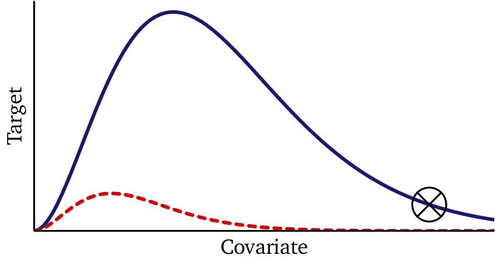
If the noise scale were known to be small, this single observation would necessitate a very high temperature, such that the curve passes close to the observed point, as shown with the blue line in the plot above. However, we may know from domain knowledge or from the other datasets that such high temperatures are a priori very unlikely. And wildly adjusting the model to fit single data points, especially in the tail of the distribution, is a classic sign of over-fitting.
On the other hand, if the noise scale were known to be comparable to the observed y-value, then a lower-temperature solution like the red curve would also be permissible: the high y-value would be explained by the noise, rather than by the curve itself. Though the red curve does not fit the data as well as the blue curve, if the data is noisy, the difference in likelihood may be negligible. And we may know from other information that it is a much more plausible solution. With only a single data point, there is no way to know which solution to prefer: disambiguating requires knowledge from other sources. This is precisely what hierarchical Bayesian models provide.
Takeaway
Some parameters, like measurement noise, are naturally shared across datasets. Modeling them globally prevents overfitting and ensures even sparse datasets can make reliable estimates.
3.3 Likelihood
With the priors in place, we now define how the observed data are generated. Each dataset follows the same physical law — Planck’s law in our example — but with its own dataset-specific parameter Ti and a shared noise scale σ.
For dataset i, the likelihood of each observation is:
\[ y_{ji} = \frac{\nu_{ji}^3}{e^{\nu_{ji} / T_i} - 1} + \epsilon, \quad \epsilon \sim \mathcal{N}(0, \sigma^2) \]
where:
- j indexes observations within dataset i,
- \(\nu_{ji}\) is the input frequency,
- Ti is the dataset-specific temperature parameter, and
- σ is the global noise parameter shared across all datasets.
This equation says that the expected response at frequency \(\nu_{ji}\) is given by Planck’s law with temperature Ti, and the observed value \(y_{ji}\) deviates from this expectation due to Gaussian noise with scale σ.
By combining this likelihood with the priors from Sections 3.1 and 3.2, we arrive at a fully specified probabilistic model:
- Dataset-specific parameters: \(T_i \sim \text{Gamma}(\alpha, \beta)\)
- Shared noise: \(\sigma \sim \text{Exponential}(1)\)
- Observations: \(y_{ji} \sim \mathcal{N} \left(\tfrac{\nu_{ji}^3}{e^{\nu_{ji}/T_i}-1}, \sigma^2\right)\)
This structure captures both dataset-level variation (through the Ti) and global uncertainty (through σ), linking them together in a coherent Bayesian hierarchy.
Takeaway
The likelihood ties priors to observed data. In our case, Planck’s law defines the expected curve per dataset, while Gaussian noise accounts for random variation around it.
3.4 Full PyMC Implementation
Now that we’ve defined the priors and likelihood, we can put everything together into a full Bayesian hierarchical model using PyMC, a Python library for probabilistic programming and inference.
The implementation below mirrors the structure we just described:
import pymc as pm
import numpy as np

# Assume we have multiple datasets: (vs[i], ys[i]) for dataset i
num_datasets = len(vs)
coords = {
    "dataset": 1+np.arange(num_datasets)
}

with pm.Model(coords=coords) as hierarchical_model:

    # Hyperpriors for the Gamma distribution controlling T
    ɑ = pm.Exponential('ɑ', scale=1)
    β = pm.Exponential('β', scale=1)

    # Alternative (and weakly-informative) choices:
    # ɑ = pm.HalfNormal('ɑ', sigma=2) or ɑ = pm.Gamma('ɑ', alpha=2, beta=1)
    # β = pm.HalfNormal('β', sigma=2) or β = pm.Gamma('β', alpha=2, beta=1)

    # Dataset-specific T values drawn from a Gamma prior
    T = pm.Gamma('T', alpha=ɑ, beta=β, size=num_datasets, dims="dataset")

    # Shared noise parameter across all datasets
    σ = pm.Exponential('σ', scale=1, initval=5)

    # Model each dataset separately
    for i in range(num_datasets):
        y_1 = pm.Deterministic(f'y_1_{i}',
                               vs[i]**3 / (pm.math.exp(vs[i] / T[i]) - 1))

        # the "observed" y has noise.  model it as Gaussian noise with scale σ
        y_obs = pm.Normal(f'y_obs_{i}', mu=y_1, sigma=σ, observed=ys[i])

     # more advanced: account for the fact that data is truncated
     # y_latent = pm.Normal.dist(mu=y_1, sigma=σ,)
     # obs = pm.Truncated("obs", y_latent, lower=0, upper=50, observed=y)


# Perform inference
with hierarchical_model:
    trace = pm.sample(chains=4, cores=2)
Let’s unpack the key components:
- Hyperpriors (α, β): These govern the Gamma distribution from which each dataset’s Ti is drawn. By learning α and β, the model infers the population-level distribution of temperatures.
- Dataset-specific parameters (T): Each dataset receives its own Ti, but the hierarchical prior links them together through the shared hyperparameters.
- Shared noise parameter (σ): A single Exponential prior defines the noise scale for all datasets, reflecting the assumption of a common measurement process.
- Likelihood: For each dataset, the expected function is defined by Planck’s law, and the observed values are modeled as Gaussian deviations around that expectation.
- Inference: Finally, we call
pm.sample()to run posterior inference using Markov Chain Monte Carlo (MCMC). This produces samples from the full posterior distributions of all parameters, allowing us to quantify both values and uncertainties.
This PyMC implementation directly encodes the hierarchical structure: dataset-specific parameters are tied together by hyperpriors, while a shared noise parameter stabilizes inference across datasets. The result is a full probabilistic model that captures both structure and uncertainty.
If you compare the code to our hypernetwork definition from Part I, the Bayesian model is simpler and easier to reason about. We will also see in the next section that it is considerably more powerful to boot.
Takeaway
A Bayesian hierarchical model can be implemented compactly in PyMC. Hyperpriors capture population-level structure, dataset parameters reflect local variation, and MCMC provides full posterior distributions.
4. Results
With the Bayesian hierarchical model defined, we can now evaluate its performance on the same synthetic datasets used in the hypernetwork experiment. Each dataset has its own hidden temperature parameter Ti, while the noise scale σ is shared across all datasets.
4.1 Training Performance
The figure below shows the model fit across the same 20 training datasets that we saw in Part I:
- Blue solid curve: the true function from Planck’s law.
- Black points: observed data for each dataset.
- Red dashed curve: posterior mean prediction from the Bayesian model.
- Red shaded regions: 80% and 50% posterior credible intervals.
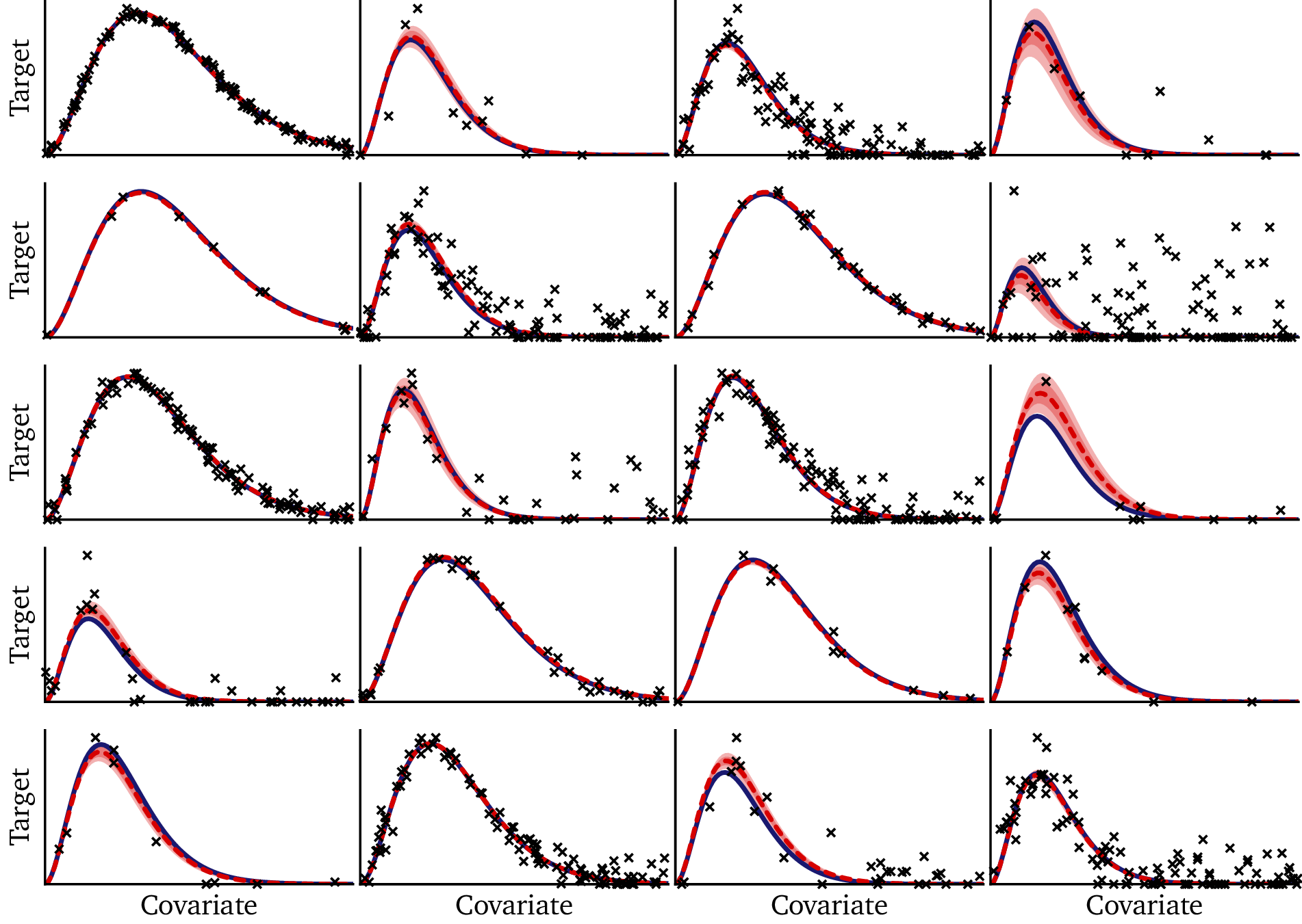
The results are striking. Even when data are sparse or noisy, the model resists overfitting. In all 20 cases, the true solution lies well within the 80% credible interval: the Bayesian model not only provides accurate solutions, but it correctly calibrates its uncertainty in each case. On larger datasets, the confidence intervals are narrow — often thinner than the plotted line — demonstrating that the model has high confidence when it is supported by ample data. On smaller or noisier datasets, the intervals widen appropriately, reflecting greater uncertainty.
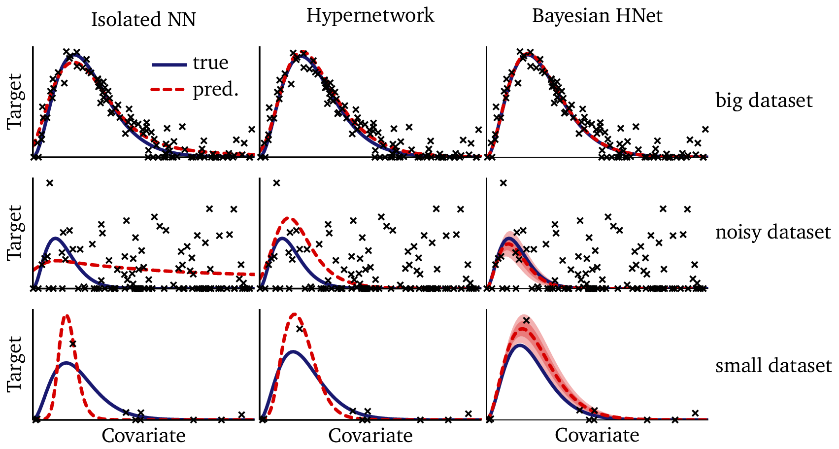
Now that we’ve tested three different technologies on the exact same problem, it’s instructive to take a minute to compare them side-by-side. In the following figure, I’ve pulled out three illustrative examples from the training data: we have a big dataset, a noisy dataset, and a small dataset. For each one, I show the training results from the isolated neural network, the hypernetwork, and the Bayesian hierarchical network:
We can see that, when given a big dataset, all of the technologies perform well. If you squint and examine the plots in detail, the hypernetwork and Bayesian network do outperform the isolated neural network; however, any of these techniques would suffice for fitting the data in this regime. With the noisy dataset, however, we see the isolated neural network fails to give a reasonable solution: it draws a line through the data, but without access to shared knowledge from the other datasets, it has no way to “know” what a reasonable solution looks like. The hypernetwork and the Bayesian network perform much better in this example, though the Bayesian network is more faithful to the true solution. In the small dataset example, we see the neural networks over-fit: one point in this dataset is off the trend due to noise. The flexible neural network models stretch and strain the solution to run through that point. The Bayesian model, on the other hand, is more circumspect: it places that point at the edge of its 80% confidence interval, favoring a solution which is closer to the true solution.
4.2 Out-of-Sample Predictions
Next, we test the model on datasets generated outside the training distribution — the same challenge where the hypernetwork showed noticeable instability.
Here, the Bayesian model performs exceptionally well. It quickly locks onto the correct functional form, even under challenging conditions, and produces credible intervals that meaningfully reflect uncertainty. Instead of diverging or producing unstable predictions, the model provides a range of plausible outcomes consistent with the generative process.
Where the hypernetwork sometimes drifted or produced unstable extrapolations, the Bayesian model generalized consistently — offering both stability and interpretable uncertainty.
4.3 Comparison with the Hypernetwork
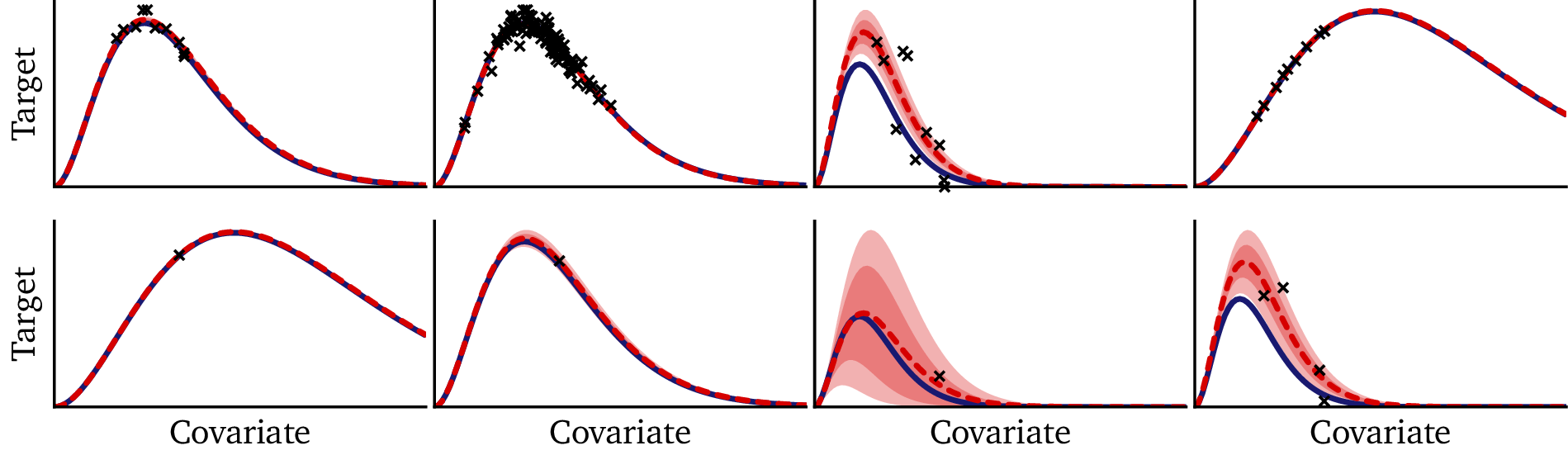
Finally, we can compare the Bayesian model directly to the hypernetwork on a few of these out-of-sample prediction tasks:
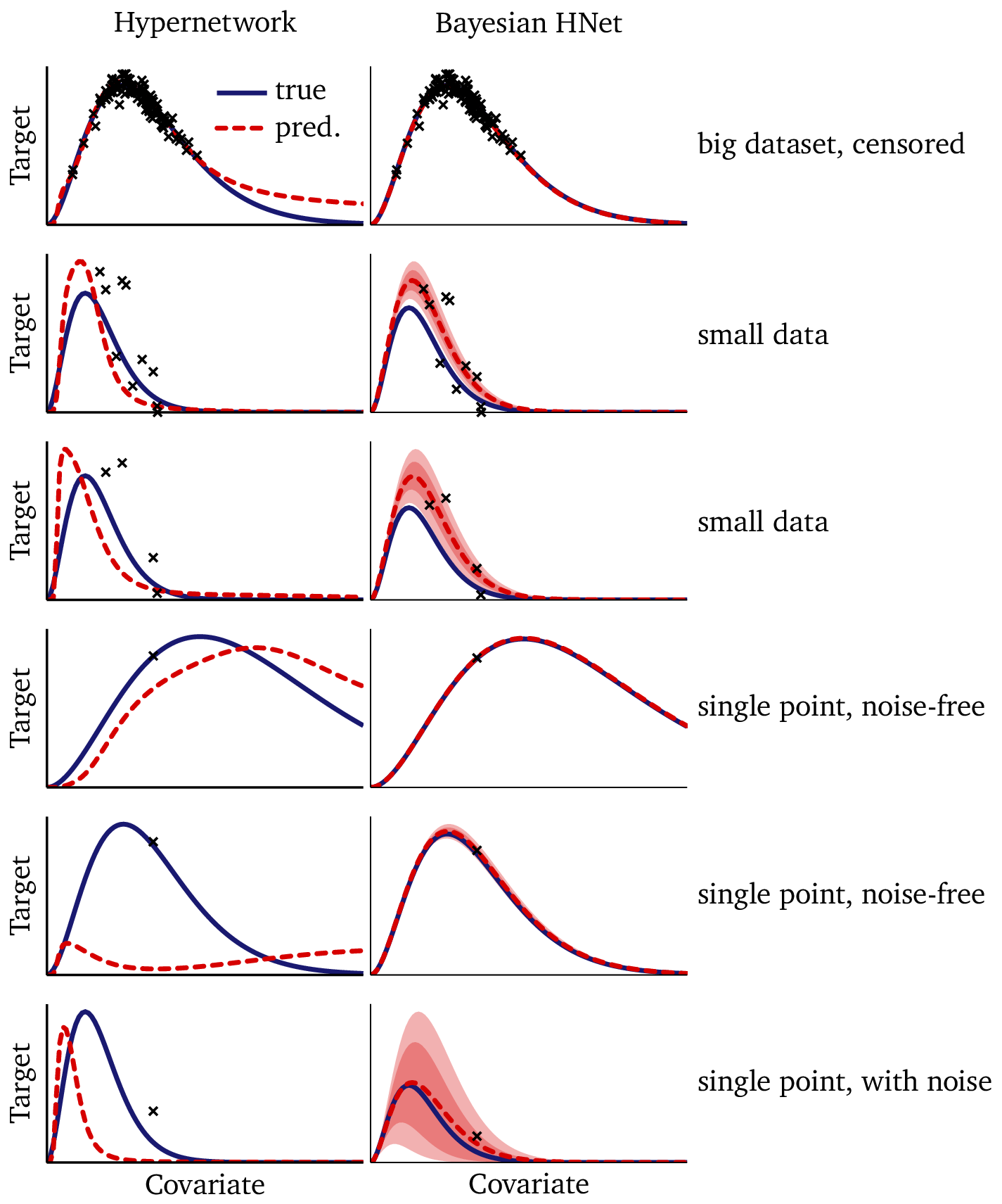
In the big-but-censored dataset (1st row), there is ample data to constrain the temperature, but there is no data in the tail. Without a fixed functional form, the flexible hypernetwork diverges from the true solution where it is unconstrained by the data. The Bayesian model, on the other hand, benefits from its prescriptive mathematical structure, which enables it to extrapolate accurately well beyond the data, provided that the temperature is known. The model prediction is essentially indistinguishable from the true solution.
We see the hypernetwork perform admirably on the small datasets (2nd and 3rd rows), especially since a normal neural network cannot perform at all on out of sample datasets like these. At the same time, the improved stability and uncertainty quantification of the Bayesian model are also clearly evident.
The high-signal, single-point datasets (4th and 5th rows) demonstrate that a single point is simply not enough information to constrain the hypernetwork: we cannot reasonably infer our embedding from a single data point. On the other hand, the structure built into our Bayesian model, which takes advantage of structure within the data (see §3.2) enables the Bayesian model to perform astoundingly well here; its performance in this regime seems almost magical, making essentially perfect predictions from single-point datasets!
The low-signal, single-point dataset in the final row is an under-constrained task which is nearly impossible in machine learning. Nonetheless, the uncertainty quantification of the Bayesian model is helpful here: while the hypernetwork simply throws out a guess, the Bayesian model tells you that it doesn’t know the solution. (N.B.: The Bayesian model happens to give an accurate solution in this example; however, the wide confidence interval tells us that this is by chance, and that we should not interpret it as a signal of high accuracy in this regime.)
The differences are clear:
- Stability: Bayesian predictions remain close to the true function across datasets, while the hypernetwork sometimes drifts.
- Noise resistance: Bayesian inference smooths through noisy observations, while the hypernetwork may overfit small fluctuations.
- Small data: Bayesian pooling across datasets prevents overfitting when data are scarce; the hypernetwork is more vulnerable.
- Uncertainty quantification: Bayesian models provide credible intervals; the hypernetwork outputs only point estimates.
Takeaway
While hypernetworks are powerful and scalable, Bayesian hierarchical models offer superior robustness, interpretability, and uncertainty quantification, particularly in small-data and out-of-sample scenarios.
5. Conclusion & Looking Ahead
Bayesian hierarchical models offer a principled way to handle hierarchical data. By combining dataset-specific parameters, shared priors, and explicit uncertainty quantification, they provide models that are both flexible and interpretable. Compared to hypernetworks, Bayesian models shine in small-data and noisy settings, where pooling information and reasoning about uncertainty are critical.
At the same time, Bayesian inference can be computationally demanding, especially for large datasets or complex models. Hypernetworks, by contrast, scale more efficiently, taking advantage of modern hardware and optimization techniques. The choice between these approaches depends on the problem: when robustness and uncertainty matter most, Bayesian models are often the better fit; when scalability and speed are paramount, hypernetworks may be preferable.
Since I used the same function in the Bayesian model that I also used to generate the data, you might suspect that the advantages the Bayesian model shows here result from simple cheating: that the correct solution is somehow baked into the model. In the next post, I will show that this is not the case: I will show that the advantages I have shown are inherent in the technique and that other, less prescient modeling choices can yield equally good results if implemented reasonably.
Takeaway
Bayesian models shine in robustness and uncertainty quantification, while hypernetworks shine in scalability. Each is valuable, but together they illustrate complementary strategies for tackling hierarchical data.